PID Process Control
In short
PID process control is a closed-loop method that continuously measures a process variable such as temperature, pressure, flow, tension or level and adjusts an output based on its difference from the setpoint. The output is calculated from a term proportional to the error (P), the accumulated error over time (I) and the rate of change of the error (D), and is applied to a valve, a heater or the speed reference of a pump or fan drive. ONX Control builds these loops in CODESYS, tuning anti-windup, feed-forward, cascade structure and filtering to the process, and commissions them together with drives and remote I/O.
How it works
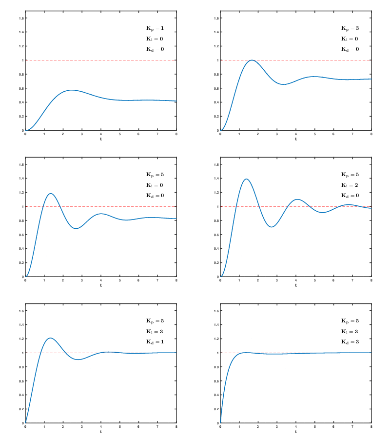
The proportional (P) term produces an output proportional to the error; used alone, load changes leave a permanent offset. The integral (I) term removes this offset by accumulating the error over time; but if the sum keeps growing while the output is saturated at its limit, overshoot and long oscillation follow. This is called integral windup and is prevented with anti-windup (stopping or back-calculating the integral at the limit). The derivative (D) term reacts to the rate of change of the error and acts as a brake on sudden changes; because it is sensitive to noise, it is usually calculated on a filtered measurement or not used at all.
On real machines PID alone is rarely enough. If a disturbance is known (for example an increase in line speed or a new material batch), it is added directly to the output as feed-forward, and the PID corrects only the remaining error. When a slow variable depends on a fast inner variable, a cascade is used: for example the outer loop controls pressure and the inner loop controls pump speed. Measurement noise is suppressed with a low-pass filter, the sample time is chosen relative to the process time constant, and switching between manual and automatic is done without a jump in the output (bumpless transfer).
-
1
Understand the process
Identify the measurement, the final control element and the process dynamics; observe dead time, time constant and gain from a step response.
-
2
Choose the loop structure
Select a single loop, a loop with feed-forward or a cascade; define output limits, anti-windup and the measurement filter.
-
3
Tuning
Starting parameters come from the step response or empirical methods, then are fine-tuned on the real process by balancing overshoot, settling time and noise.
-
4
Commissioning and monitoring
Setpoint, measurement and output trends are logged; behaviour is verified at different operating points, and parameters are switched by operating point where needed (gain scheduling).
Critical parameters
| Parameter | Why it matters | Typical range / ONX field data |
|---|---|---|
| Line speed and process dynamics | Determine how fast the process changes, the required sample time and the need for feed-forward; process gain can also change with speed. | Defined per project |
| Control tolerance (setpoint accuracy) | The accepted steady-state offset and ripple; sensor accuracy and resolution set the limit below which control cannot go. | Defined per project |
| Response time and loop cycle time | The time to respond to a setpoint change or disturbance; the loop cycle must be clearly shorter than the process time constant. | Defined per project |
| Dead time and measurement noise | Measurement delay and noise limit the achievable gain; filter settings and whether to use the D term are decided accordingly. | Defined per project |
| Final control element and limits | The range and saturation points of the valve, heater or drive speed reference determine the anti-windup design and the controllable range. | Defined per project |
ONX architecture
In the ONX architecture PID loops run in CODESYS on an industrial PC or smart controller. The starting point is standard function blocks such as PID and PID_FIXCYCLE from the CODESYS Util library; for applications that need anti-windup, feed-forward, cascade connection, filtering and manual/automatic switching, these functions are completed with application-specific code. Sensors are read through EtherCAT remote I/O via 4-20 mA, 0-10 V or thermocouple/PT100 inputs.
Final control elements such as pumps, fans and conveyors are speed-controlled by AC drives over EtherCAT or an analog reference. Controlling pump and fan flow by speed instead of throttling a valve gives significant energy savings, because by the affinity laws power varies roughly with the cube of speed. Setpoints, parameters and trends are managed from the operator panel.

CODESYS
Standard PID function blocks, anti-windup, feed-forward, cascade loops, filtering and trend logging.

Industrial PCs and smart controllers
Industrial PC, panel PC or smart controller running CODESYS Control RTE.
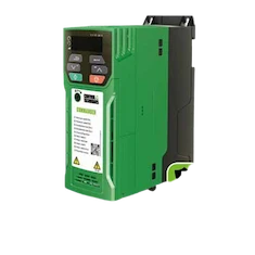
AC drives
General-purpose and high-performance AC drives as speed-controlled final control elements for pumps, fans and conveyors.

Motors
Induction motors and integrated drive motors for pump and fan drives.
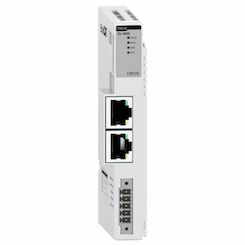
Remote I/O
Analog inputs for temperature, pressure, flow and level sensors and output modules for valves and heaters.
Field reference
The images below illustrate the principle of PID control: a closed loop in which the output is calculated from the difference between setpoint and measurement, and the same structure applied to tension control.
Principle illustrations

Retrofit scenario
A typical picture on existing machines: a separate panel-mounted temperature or process controller for each loop, flow set by throttling a valve, pumps and fans running at fixed speed, and loops whose settings are not documented. In a retrofit the sensors and valves are usually kept; the loops are brought together in one CODESYS controller, drives are added to pumps and fans, and setpoints are linked to recipes.
- Recording existing loops, sensors, valves and controller settings
- Evaluating a move from valve throttling to drive speed control on pumps and fans
- Moving the loops to CODESYS with anti-windup, feed-forward and, where needed, cascade structure
- Collecting sensor signals through EtherCAT remote I/O
- Commissioning with step tests, trend logging and tuning at different operating points
Frequently asked questions
What do the P, I and D terms do?
The P term makes a correction proportional to the error, the I term removes steady-state offset by accumulating the error over time, and the D term reacts to the rate of change of the error to reduce overshoot on sudden changes. PI is enough for many processes; the D term is used carefully, with filtering, on noisy measurements.
What is integral windup (anti-windup)?
If the integral term keeps growing while the output is at its limit (for example a fully open valve), the output stays saturated long after the error changes sign and a large overshoot follows. Anti-windup prevents this by stopping or back-calculating the integral while the output is at its limit.
When is cascade control used?
Cascade control is used when the controlled variable is slow and an intermediate variable that affects it is fast. For example the outer loop controls pressure and the inner loop controls pump speed; the inner loop corrects disturbances before the outer loop notices them.
How are PID parameters tuned?
First a step response is taken to identify dead time, time constant and gain; starting values are calculated from this or from empirical methods. They are then fine-tuned on the real process by balancing overshoot, settling time and noise. On processes whose operating point varies widely, parameters are switched by operating point.
Should PID run inside the drive or in the PLC?
For simple applications such as pressure control of a single pump, the drive's built-in function may be enough. On machines where several loops interact, need feed-forward or cascade structure and are managed by recipe, bringing the loops together in CODESYS is tidier for tuning, monitoring and maintenance.
Discuss your process control project with our engineers
Share the variables you want to control, the sensors and the final control elements; we will come back with a loop structure and hardware proposal.